
solution
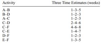
For the activity data related to a small project, as shown, draw the PERT chart and find
a. the critical path and its expected time
b. the slack in all other paths
c. the standard deviation associated with the project end date
Design a cost monitoring report that expands the data provided in Table 4.1.
You are at the 18-month point of a 24-month project with a $400,000 budget. The schedule variance has been estimated as $30,000 and the cost variance as $20,000. The BCWS is $300,000.
a. ACWP
b. BCWP
c. ECAC
d. ETAC
Compare these results with those in the EVA example in the text. Why are they different?
In general, for a project:
a. If BCWP > BCWS, is the project early or late? Explain.
b. If ACWP > BCWP, is the project over or under cost? Explain.
c. If ACWP
"Looking for a Similar Assignment? Get Expert Help at an Amazing Discount!"