
solution
Juniper Networks to Benefit From Digital India Programme
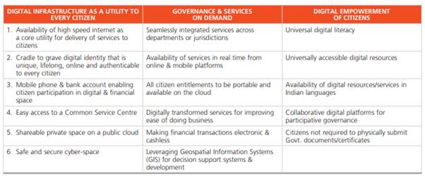
Juniper Networks is an American multinational corporation headquartered in Sunnyvale, California that develops and markets networking products. Its products include routers, switches, network management software, network security products and software-defined networking technology. Company competes with Cisco, Ciena and Hewlett-Packard, among others. The NYSE-listed company has invested $1 billion in India in the past six years, mostly on research and development, and has about 2,600 workers in the country across locations including Bengaluru and Delhi. Juniper Networks is planning to invest $1 billion more in the Indian operations to tap into the opportunities which will arise from India’s digital transformation led by cloud-based services. The company wants to be part of Government of India’s digital vision. The Digital India programme is centred on three key vision areas:
"Looking for a Similar Assignment? Get Expert Help at an Amazing Discount!"